

MDF, CAN & Calibration Data
Vehicle and engine testing produces MDF files, CAN bus logs and calibration data. UniPlot imports all of them through add-ins that convert the data into its NC2 format, so measured signals, decoded CAN signals and calibration maps can be plotted and compared side by side. Engine maps get their own tools: contour plots with isolines, 3D surfaces, cross-sections, full load lines and difference maps.
The add-ins are activated once with Tools=>Add-In Manager.
Guides
Open .mf4 files, including CAN bus logging data.
Turn BLF and ASC log files into physical signals.
Use an AUTOSAR network description instead of a DBC.
Create MDF4 files from a UniScript script.
Quick answers
How do I import MDF 3.x files, for example from INCA?
Load the MDF Import (e.g. VS100/INCA) add-in, then choose
File=>Import Data with the file type MDF File (*.dat; *.mdf). This
reads MDF files up to version 3.3 as written by INCA/VS100, the IAV Drive
Recorder or CANalyzer. See Import of MDF Files. See also
A .dat/.mf4 file opens in ETAS INCA MDA but UniPlot reports “Import filter ‘_DoImportVS100File’ failed” or crashes. Why?.
Can UniPlot read Vector ASC log files?
Yes, with the CAN Import add-in and the file type
Vector CAN Log (*.blf; *.asc). Classical and CAN FD records are read; the
header (up to 50 lines) is stored as global attributes of the NC2 file. The
signals are decoded with the DBC or ARXML files of the active CAN
configuration, see How do I decode a CAN log file (BLF or ASC) with a DBC file?.
Are CAN FD frames in ASC files supported?
Yes, since R2022.4. Besides classical records, the import reads CAN FD
records of the form
<time> CANFD <channel> <dir> <id> <brs> <esi> <dlc> <data_len> <data>.
Other record types in the file are ignored. In BLF and MF4 files only
classical CAN frames are evaluated. See also Does UniPlot support CAN FD, also in BLF and MF4 bus logging files?.
Can UniPlot decode multiplexed CAN messages?
Yes. Signals that share one message Id through a multiplexer are decoded as defined in the DBC file. Since R2024.3 the multiplexer itself is also written to the NC2 file. See also BLF import shows no channels (“Files does not contain any channels”), all values are zero, or signals are missing. What should I check?.
How do I import only some of the CAN messages?
In Tools=>CAN Configuration (DBC file), check only the messages you need. All signals of a checked message are converted, unchecked messages are skipped. At least one and at most 800 messages can be selected.
How do I import CAN data from one bus only?
In the CAN configuration, choose a bus number (1 to 255) for each DBC or
ARXML file instead of “all”. Only frames from that bus are read. The NC2
file records the bus in the attribute BusNumber, for example “CAN12”.
Which time channel belongs to an MDF or CAN signal?
You don’t have to find out. Choose the dataset type
2D: y/t "MDF/INCA/CAN/ODS/iFile" and select only the signal; UniPlot
picks the matching time channel. For MDF 3.x files you can even combine
signals from different time groups, UniPlot interpolates them to a common
time base. See also A BLF signal is displayed at a lower sample rate than it was recorded, or fast state changes are missing. How can I show the real sampling?.
How do I get shorter channel names from MDF files?
Tools=>MDF Configuration (INCA) sets how channel names are built for
MDF 3.x files: strip the group name (G1_), the device name after the
backslash or the CAN Id (_CANxx), or use the MDF display identifier as
channel name. See Configuration. See also
Where do I find the MDF import settings for channel names, for example to remove the device suffix _ETK_1?.
Are the trigger times of an MDF file kept?
Yes, for MDF 3.x files. If the measurement used triggers, each time channel
gets the attributes tr_trig_time, tr_trig_pre, tr_trig_post,
tr_condition and tr_wincount (the number of trigger events).
How do I convert MDF files to NC2?
Every import converts the file: File=>Import Data writes an NC2 file
that can later be opened directly. In a script, auto_ImportData(ssFile)
does the conversion and returns the name of the NC2 file, so a loop
converts a whole directory. See also What does Delayed Channel Import do, and how can I speed up the import of very large MF4/MDF files?.
How do I import DCM calibration files?
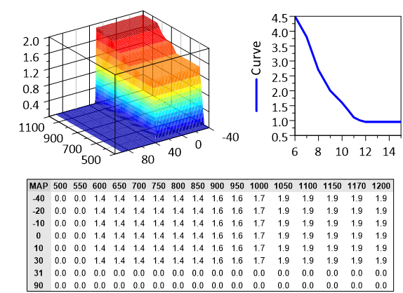
Load the add-in Calibration Data import (v1.0) and choose
File=>Import Data with the type
Calibration Data File (*.dcm;*.DCM;*.xml). DCM version 2.0 is
supported. The dataset type Calibration Plot (1D, 2D, 3D) draws single
values, curves and maps with their axes; Calibration Table (1D, 2D, 3D)
shows the values as a table. See
Import of Calibration Data Files. See also How can I read DCM or PACO calibration data files exported from INCA?.
Can UniPlot read PaCo calibration files?
Yes, with the same Calibration Data add-in and file type as DCM files. PaCo
files are XML files, so select them with the extension .xml. Maps,
curves and single values are plotted in the same way.
How do I compare two versions of a map?
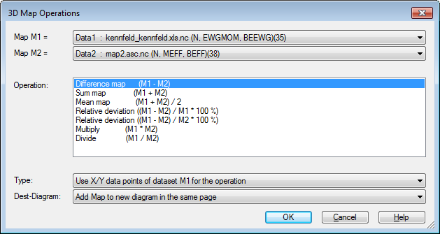
Load both maps into one page, right-click an isoline of one map and choose
3D-Difference (or Data=>More Data Functions => Difference map and
other functions). Select map M1 and M2 and the operation, for example
M1-M2. UniPlot creates a new map of the difference. See
Data=>Difference map and other functions (3D). See also
How do I create a difference dataset or difference map, and why does it fail or give no result?.
How do I show a map as a filled contour plot?
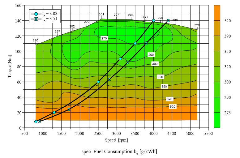
Create a 3D dataset (x, y, z channel), for example by choosing the type
3D: x/y/z in the import dialog. UniPlot interpolates the points and
draws isolines. Isoline values, fill colors and the option Color Filling
between Isolines are set in Data=>3D-Dataset=>Color Map. See also
How do I colour an X/Y/Z map with a colour map, change the isolines and add a colour legend?.
How do I show a map as a 3D surface?
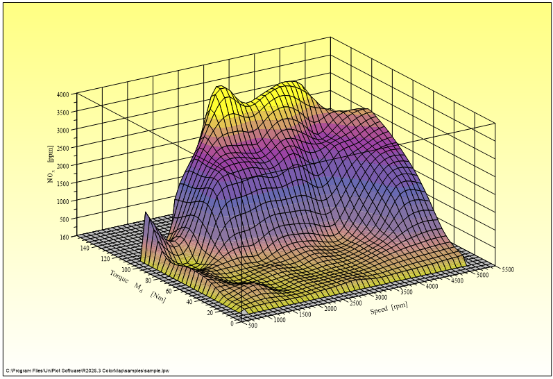
Select the 3D dataset and choose Data=>3D-Dataset=>3D Surface / Bars for the surface style (mesh, fill color, color gradient). The viewing angle is set with Diagram=>3D View.
How do I get cross-sections of a map?
Select the map and choose Data=>More Data Functions, then Cross-section for Y = constant (Profile) or Cross-section for X = constant (Profile). Enter the section values separated by semicolons; UniPlot creates a new page with one curve per section, optionally color filled. A cross-section along any 2D curve is available as well. See Data=>Cross-section (3D).
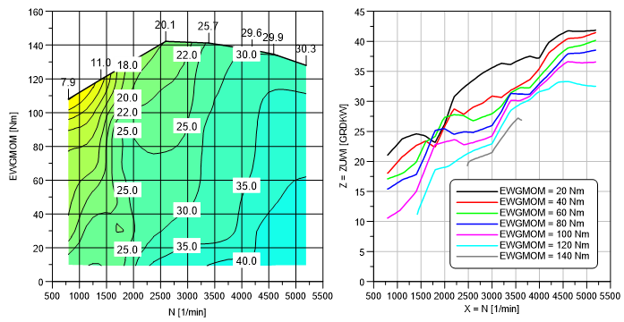
How do I add the full load line (WOT) to a map?
Data=>More Data Functions => Find data hull (WOT Curve) (or Find Data Hull in the context menu of an isoline) calculates the full load line from the measured points and saves it as the hull of the map. In Data=>3D-Dataset=>Hull choose North Line to draw only the full load line and clip the isolines there. A measured full load curve in the same page can also be turned into the hull with the isoline context menu command Convert 2D-Curve to Hull. See also How do I fit, remove or define the hull (envelope) of a 3D map?.
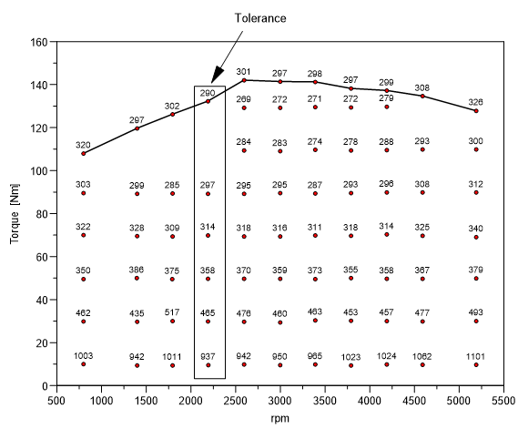
Can UniPlot draw a map from points that are not on a grid?
Yes. Data=>Interpolation calculates an equidistant grid of 5 to 100 rows and columns from the measured points and sets the interpolation method. As a rule of thumb, 100 to 200 evenly distributed points give an accurate map with a 30 x 30 grid. See also My 3D map shows local minima or maxima that do not exist in the data. How can I avoid this?.
How do I choose which isolines are drawn?
In Data=>3D-Dataset=>Color Map enter single values, or a range as
Minimum, Delta, Maximum: 100,10,130 creates the isolines 100, 110,
120 and 130. Up to 99 values are possible, each with its own line style and
fill color. See also How do I set the isoline range or colour map for many 3D plots at once?.
How do I see where one consumption map is better than another?
Use the difference map (see the question above) with the operation
(M1-M2)/M1 * 100%: the result is a map of the relative deviation in
percent, so improvements and losses are visible at a glance.
How do I turn a measured map into a calibration table?
The Map-Calculator add-in calculates a matrix with the row and column values you specify from a measured 3D dataset and saves it as INCA-CSV, DAMOS, Magneti-Marelli-CSV, text or Excel file, or copies it to the clipboard. See Map Calculator. See also How do I fit, remove or define the hull (envelope) of a 3D map?.
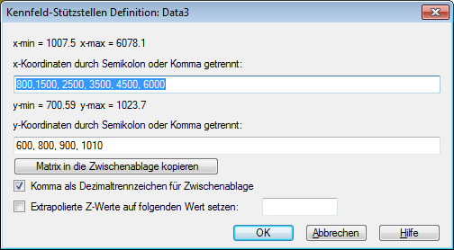
How do I calculate a channel from a map for a measurement?
The isoline context menu command Map-Calculator: Interpolate Z-Channel reads the x and y channels of a data file, for example speed and torque of a drive cycle, looks up the z value in the selected map and saves it as a new channel in the NC file. Points outside the map can be set to missing.
Support questions
Error messages, settings and other practical problems in this area are answered in the FAQ: Data Import and File Formats and Diagrams, Axes and 3D Maps.